5. Training a reflectorch model

First, we import the necessary methods from the reflectorch package, as well as other basic Python packages:

import matplotlib.pyplot as plt
import numpy as np
import torch

from reflectorch import SAVED_MODELS_DIR, SaveBestModel, StepLR, get_trainer_by_name, get_callbacks_by_name
from reflectorch.extensions.jupyter import JPlotLoss

Tip

Alternatively, we can import everything from reflectorch with from reflectorch import *

5.1. The training loop

5.1.1. Loading the trainer

For training a model we use the Trainer class, which contains all the components necessary for the training process such as the data generator, the neural network and the optimizer.

We can initialize the trainer according to the specifications defined in a YAML configuration file using the get_trainer_by_name method which takes as input the name of the configuration file. If the package was installed in editable model, the configuration files are read from the configs directory located inside the repository, otherwise the path to the directory containing the configuration file should also be specified using the config_dir argument. The load_weights argument should be set to False since we want the neural network weights to be randomly initialized for a fresh training.

config_name = 'a_base_point_xray_conv_standard'
trainer = get_trainer_by_name(config_name, load_weights=False)

Model a_base_point_xray_conv_standard loaded. Number of parameters: 5.02 M

The trainer contains several important attributes we can inspect:

1. The Pytorch optimizer. We can observe that the optimizer specified in the configuration is AdamW:

trainer.optim

AdamW (
Parameter Group 0
    amsgrad: False
    betas: [0.9, 0.999]
    capturable: False
    differentiable: False
    eps: 1e-08
    foreach: None
    fused: None
    lr: 0.001
    maximize: False
    weight_decay: 0.0005
)

Note

The learning rate can be easily changed using trainer.set_lr(new_lr)

2. The batch size

trainer.batch_size

4096

3. The Pytorch neural network module. We can see that the network is an instance of the class NetworkWithPriors. This architecture consists of a multilayer perceptron (MLP) with residual connections, batch normalization layers and GELU activations (trainer.model.mlp). An embedding network, here a 1D CNN (trainer.model.embedding_net), produces a latent embedding of the input batch of reflectivity curves which is concatenated with the prior bounds for the thin film parameters.

trainer.model

NetworkWithPriors(
  (embedding_net): ConvEncoder(
    (core): Sequential(
      (0): Sequential(
        (0): Conv1d(1, 32, kernel_size=(3,), stride=(2,), padding=(1,))
        (1): BatchNorm1d(32, eps=1e-05, momentum=0.1, affine=True, track_running_stats=True)
        (2): GELU(approximate='none')
      )
      (1): Sequential(
        (0): Conv1d(32, 64, kernel_size=(3,), stride=(2,), padding=(1,))
        (1): BatchNorm1d(64, eps=1e-05, momentum=0.1, affine=True, track_running_stats=True)
        (2): GELU(approximate='none')
      )
      (2): Sequential(
        (0): Conv1d(64, 128, kernel_size=(3,), stride=(2,), padding=(1,))
        (1): BatchNorm1d(128, eps=1e-05, momentum=0.1, affine=True, track_running_stats=True)
        (2): GELU(approximate='none')
      )
      (3): Sequential(
        (0): Conv1d(128, 256, kernel_size=(3,), stride=(2,), padding=(1,))
        (1): BatchNorm1d(256, eps=1e-05, momentum=0.1, affine=True, track_running_stats=True)
        (2): GELU(approximate='none')
      )
      (4): Sequential(
        (0): Conv1d(256, 512, kernel_size=(3,), stride=(2,), padding=(1,))
        (1): BatchNorm1d(512, eps=1e-05, momentum=0.1, affine=True, track_running_stats=True)
        (2): GELU(approximate='none')
      )
    )
    (avpool): AdaptiveAvgPool1d(output_size=1)
    (fc): Linear(in_features=512, out_features=128, bias=True)
  )
  (mlp): ResidualMLP(
    (first_layer): Linear(in_features=128, out_features=512, bias=True)
    (blocks): ModuleList(
      (0-7): 8 x ResidualBlock(
        (activation): GELU(approximate='none')
        (batch_norm_layers): ModuleList(
          (0-1): 2 x BatchNorm1d(512, eps=0.001, momentum=0.1, affine=True, track_running_stats=True)
        )
        (condition_layer): Linear(in_features=16, out_features=1024, bias=True)
        (linear_layers): ModuleList(
          (0-1): 2 x Linear(in_features=512, out_features=512, bias=True)
        )
      )
    )
    (last_layer): Linear(in_features=512, out_features=8, bias=True)
  )
)

5.1.2. Defining callbacks

We can control the training process using callback objects, such as:

1. JPlotLoss - allows the interactive visualization of the loss curve when training inside a Jupyter Notebook, the frequency argument setting the refresh rate of the interactive widget

2. StepLR - implements a learning rate scheduler which decreases the learning rate in steps (after a number of iterations defined by step_size the learning rate is multiplied by the factor gamma). Other types of learning rate schedulers can alternatively be used, such as CosineAnnealingWithWarmup, LogCyclicLR, OneCycleLR or ReduceLROnPlateau.

3. SaveBestModel - it enables the periodic saving of the weights of the neural network during training. After a number of iterations defined by the freq argument, the weights of the neural network are saved at the specified path if the current average loss (computed over the last average iterations) is lower than the loss for the previous save. The history of the losses and learning rate values is also saved.

When the package is installed in editable mode, the default save path is relative to the repository directory (defined by the global variable SAVED_MODELS_DIR).

save_model_name = 'model_' + config_name + '.pt'
save_path = str(SAVED_MODELS_DIR / save_model_name)

We group the callback objects together in a touple:

callbacks = (
    JPlotLoss(frequency=10), 
    StepLR(step_size=5000, gamma=0.1, last_epoch=-1), 
    SaveBestModel(path=save_path, freq=100, average=10),
)

Note

The callbacks can also be initialized directly from the configuration file: callbacks = get_callbacks_by_name(config_name)

5.1.3. Run the training

The training process is initiated by calling the train method of the trainer. This method accepts as arguments the previously defined tuple of callbacks, as well as the number of iterations (batches). Notably, a new batch of data is generated at each iteration, the training taking place in a “one-epoch regime”.

trainer.train(num_batches=1000, callbacks=callbacks)

After training, the history of the losses and learning rates can be accessed via trainer.losses and trainer.lrs. We can also find them together with the model state_dict in the saved dictionary:

torch.load(save_path, weights_only=False).keys()

dict_keys(['model', 'lrs', 'losses', 'prev_save', 'batch_num', 'best_loss'])

Tip

The saved weights can be loaded into a compatible neural network (net) as:

saved_dict = torch.load(save_path)
model_state_dict = saved_dict['model']
net.load_state_dict(model_state_dict)

The model state dictionaries of all the saved ‘.pt’ files in a directory can be further converted to the ‘.safetensors’ format for exporting to Huggingface using the convert_pt_to_safetensors method.

5.1.4. Training from the terminal

Above we described the workflow for training a model in a Jupyter Notebook, where we loaded the trainer from the configuration file but defined the callbacks manually. Alternatively, one can train a model from the terminal (in this case the callbacks defined in the configuration file are used):

python -m reflectorch.train config_name

5.2. Customizing the YAML configuration for training

In the following we show how the YAML configuration file can be customized.

Sample YAML configuration

general:
  name: a_base_point_xray_conv_standard
  root_dir: null
  
dset:
  cls: ReflectivityDataLoader
  prior_sampler:
    cls: SubpriorParametricSampler
    kwargs:
      param_ranges:
        thicknesses: [1., 500.]
        roughnesses: [0., 60.]
        slds: [0., 50.]
      bound_width_ranges:
        thicknesses: [1.0e-2, 500.]
        roughnesses: [1.0e-2, 60.]
        slds: [1.0e-2, 5.]
      model_name: standard_model
      max_num_layers: 2
      constrained_roughness: true
      max_thickness_share: 0.5
      logdist: false
      scale_params_by_ranges: false
      scaled_range: [-1., 1.]
      device: 'cuda'
      
  q_generator:
    cls: ConstantQ
    kwargs:
      q: [0.02, 0.15, 128]
      device: 'cuda'
      
  intensity_noise:
    cls: GaussianExpIntensityNoise
    kwargs:
      relative_errors: [0.01, 0.3]
      consistent_rel_err: false
      apply_shift: true
      shift_range: [-0.3, 0.3]
      add_to_context: true

  curves_scaler:
    cls: LogAffineCurvesScaler
    kwargs:
      weight: 0.2
      bias: 1.0
      eps: 1.0e-10

model:
  network:
    cls: NetworkWithPriors
    pretrained_name: null
    device: 'cuda'
    kwargs:
      embedding_net_type: 'conv'
      embedding_net_kwargs:
        in_channels: 1
        hidden_channels: [32, 64, 128, 256, 512]
        kernel_size: 3
        dim_embedding: 128
        dim_avpool: 1
        use_batch_norm: true
        use_se: false
        activation: 'gelu'
      pretrained_embedding_net: null
      dim_out: 8
      dim_conditioning_params: 0
      layer_width: 512
      num_blocks: 8
      repeats_per_block: 2
      residual: true
      use_batch_norm: true
      use_layer_norm: false
      mlp_activation: 'gelu'
      dropout_rate: 0.0 
      conditioning: 'film'
      concat_condition_first_layer: false
       
training:
  trainer_cls: PointEstimatorTrainer
  num_iterations: 10000
  batch_size: 4096
  lr: 1.0e-3
  grad_accumulation_steps: 1
  clip_grad_norm_max: null
  update_tqdm_freq: 1
  optimizer: AdamW
  trainer_kwargs:
    train_with_q_input: false
    condition_on_q_resolutions: false
    rescale_loss_interval_width: true
    use_l1_loss: true
    optim_kwargs:
      betas: [0.9, 0.999]
      weight_decay: 0.0005
  callbacks:
    save_best_model:
      enable: true
      freq: 500
    lr_scheduler:
      cls: CosineAnnealingWithWarmup
      kwargs:
        min_lr: 1.0e-6
        warmup_iters: 500
        total_iters: 10000

  logger:
    cls: TensorBoardLogger
    kwargs:
      log_dir: "tensorboard_runs/test_1"

The general key, contains the following subkeys:

• name - name used for saving the model

• root - path to the root directory, defaults to the package directory

general:
  name: a_base_point_xray_conv_standard
  root_dir: null

The dset key defines the settings pertaining to the data generation (i.e. the SLD profile parameterization, the ranges of the thin film parameters, the q values, the noise added to the reflectivity curves and the scaling of the reflectivity curves). It has the following subkeys:

1. cls (optional) - the class of the data loader. If not provided, the default class ReflectivityDataLoader is used.

2. prior_sampler - responsible for defining the type of SLD parameterization, the ranges from which the thin film parameters are sampled and the ranges from which the widths of the prior bounds are sampled. The SubpriorParametricSampler class first samples a center (C) from the parameter ranges and a width (W) from the bound width ranges. This defines a subinterval delimited by the minimum prior bound B_min = C - W/2 and the maximum prior bound B_max = C + W/2. Then, the values of the parameters (to be used for simulating the reflectivity curves and as ground truth) are uniformly sampled within the interval [B_min, B_max]. It has the following keyword arguments:

• model_name - name associated with the type of SLD parameterization. Here, standard_model represents the standard box model parameterization of the SLD with the parameters thickness, roughness and real layer SLD.

• max_num_layers - the number of layers in the thin film (in addition to the substrate)

• param_ranges - the ranges from which the values of each type of thin film parameter are uniformly sampled (for the standard model thicknesses, roughnesses and slds)

• bound_width_ranges - the ranges from which the prior bound widths of each type of thin film parameter are uniformly sampled. If the argument logdist is set to true, the prior bound widths are sampled uniformly on a logarithmic scale instead, biasing the training towards smaller prior bound widths.

• constrained_roughness - if true the sampling of the roughness parameters is constrained such that the roughness of an interface between two layers does not exceed a fraction (defined by the argument max_thickness_share) of the thickness of either one of those layers.

• max_total_thickness (optional) - if provided, the sampling is performed such that the sum of the sampled layer thicknesses does not exceed this value

• scale_params_by_ranges - if true the parameters are scaled with respect to their ranges, otherwise they are scaled with respect to their subprior bound interval. The default is false.

• scaled_range - the ML-friendly range to which the parameters (and prior bounds) are scaled to, the default is [-1, 1]

• device - default is 'cuda' for GPU use, can be changed to 'cpu' for CPU use

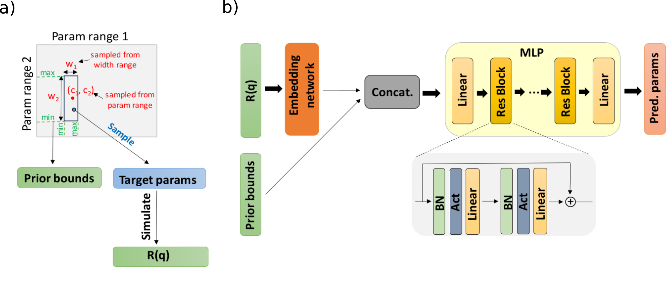
Fig. 5.1 (a) Parameter sampling process (b) Neural network architecture

dset:
  cls: ReflectivityDataLoader
  prior_sampler:
    cls: SubpriorParametricSampler
    kwargs:
      param_ranges:
        thicknesses: [1., 500.]
        roughnesses: [0., 60.]
        slds: [0., 50.]
      bound_width_ranges:
        thicknesses: [1.0e-2, 500.]
        roughnesses: [1.0e-2, 60.]
        slds: [1.0e-2, 5.]
      model_name: standard_model
      max_num_layers: 2
      constrained_roughness: true
      max_thickness_share: 0.5
      logdist: false
      scale_params_by_ranges: false
      scaled_range: [-1., 1.]
      device: 'cuda'

3. q_generator - responsible for generating the transfer vector (q) values at which the reflectivity is to be simulated. We must first specifiy its class. The ConstantQ class generates a fixed discretization for all the reflectivity curves in the batch. Its q keyword argument is a tuple formatted as [q_min, q_max, num_q_points], which defines the minimum q value, the maximum q value as well as the number of points (including the interval boundaries) to be equidistantly sampled. Other q generator classes are available such as VariableQ (equidistant grid with variable q_min, q_max and num_q_points, further described in the Advanced functionality section) and ConstantAngle which generates the grid of q values based on equidistantlly sampled scattering angles and the wavelength of the beam. The device argument can be changed to 'cpu' for CPU use (default is 'cuda' for GPU use).

dset:
  q_generator:
    cls: ConstantQ
    kwargs:
      q: [0.02, 0.15, 128]
      device: 'cuda'
      

4. q_noise (optional) - responsible for adding noise to the generated q values, which emulates possible measurement errors due to sample misalignment. The BasicQNoiseGenerator class can add both systematic q shifts (the same change applied to all q points of a curve) and random noise (different changes applied to each q point of a curve) to the q values of the batch of curves, it has the following arguments:

• shift_std - the standard deviation of the normal distribution for sampling the systematic q shifts (one value sampled per curve in the batch)

• noise_std - the standard deviation of the normal distribution for sampling the random q noise (one value sampled per point in the curve). The standard deviation is the same for all curves in the batch if provided as a float, or uniformly sampled from a range for each curve in the batch if provided as a tuple.

dset:
  q_noise:
    cls: BasicQNoiseGenerator
    kwargs:
      shift_std: 1.0e-3
      noise_std: [0., 1.0e-3]

5. intensity_noise - responsible for adding noise to the intensity values of the reflectivity curves.

   The GaussianExpIntensityNoise combines three types of noise:

   • Gaussian noise: Applies Gaussian noise to account for count-based Poisson noise as well as other sources of error.

   • Shift noise: Applies a multiplicative scaling to the curves, equivalent to a vertical shift in logarithmic space.

   • Background noise: Adds a constant background to the curves.

   It has the following arguments:

   • relative_errors - range of relative errors for Gaussian noise.

   • consistent_rel_err - if true, uses a consistent relative error for Gaussian noise across all points in a curve.

   • apply_shift - if true, applies shift noise to the curves.

   • shift_range - range of shift factors for shift noise.

   • apply_background - if true, applies background noise to the curves.

   • background_range - range for background values.

intensity_noise:
  cls: GaussianExpIntensityNoise
  kwargs:
    relative_errors: [0.01, 0.3]
    consistent_rel_err: false
    apply_shift: true
    shift_range: [-0.3, 0.3]
    apply_background: false
    background_range: [1.0e-10, 1.0e-4]
    add_to_context: true

6. smearing (optional) - responsible for adding resolution smearing to the curves (which can occur in neutron experiments due to uncertainties in incident angle or wavelength). The intensity at a q point will be the average of the intensities of neighbouring q points, weighted by a gaussian profile. The arguments of the Smearing class are:

• sigma_range - the range for sampling the resolutions

• constant_dq - if True the smearing is constant (the resolution is given by the constant dq at each point in the curve, i.e. x-ray variant), otherwise the smearing is linear (the resolution is given by the constant dq/q at each point in the curve, i.e. neutron variant)

• gauss_num - the number of points used to define the Gaussian smearing kernel. A higher number increases precision at the cost of computational efficiency.

• share_smeared - the share of curves in the batch for which the resolution smearing is applied

dset:   
  smearing:
    cls: Smearing
    kwargs:
      sigma_range: [0.01, 0.08]
      constant_dq: False
      gauss_num: 17
      share_smeared: 0.8

7. curves_scaler - responsible for scaling the reflectivity curves to a ML-friendly range. The LogAffineCurvesScaler class scales the reflectivity curves (R) accoring to the formula:

\(R_{scaled} = log_{10}(R + eps) \times weight + bias\)

The argument eps sets the minimum intensity value of the reflectivity curves which is considered. The default values of 1.0e-10 for eps, 0.2 for weight and 1.0 for bias results in the interval [-1, 1] for the scaled reflectivity curves.

dset:    
  curves_scaler:
    cls: LogAffineCurvesScaler
    kwargs:
      weight: 0.2
      bias: 1.0
      eps: 1.0e-10

The model key defines the neural network architecture. Its network subkey contains the following subkeys:

• cls - the class of the neural network

• pretrained_name - the name of a pretrained model used to initialize the weights (optional)

• device - the Pytorch device (either cuda or cpu)

• kwargs - the keyword arguments for the provided class

The NetworkWithPriors class has the following keyword arguments:

• embedding_net_type - the type of embedding network (e.g. 'conv' for a 1D CNN, 'fno' for a FNO)

• embedding_net_kwargs - the keyword arguments corresponding to the chosen embedding network (e.g. for the 1D CNN: in_channels - the number of input channels of the 1D CNN, hidden_channels - list with the number of channels for each layer of the 1D CNN, dim_embedding - the dimension of the embedding produced by the 1D CNN, dim_avpool - the output size of the adaptive average pooling layer, activation - the type of activation function in the 1D CNN)

• pretrained_embedding_net - the path to the weights of a pretrained embedding network (optional)

• dim_out - the dimension of the output produced by the MLP (i.e. the number of thin film parameters to be predicted)

• dim_conditioning_params - the dimension of extra parameters used as input to the network in specific training scenarios (such as the resolution coefficient dq/q), defaults to 0.

• layer_width - the width (i.e. number of neurons) of a linear layer in the MLP

• num_blocks - the number of residual blocks in the MLP

• repeats_per_block - the number of normalization/activation/linear repeats in a block

• use_batch_norm - whether to use batch normalization in the MLP

• use_layer_norm - whether to use layer normalization in the MLP (if batch normalization is not used)

• mlp_activation - the type of activation function in the MLP

• dropout_rate - dropout rate for each block

• conditioning - the modality in which the prior bounds are provided to the network, either by concatenating the prior bounds to the data embedding ( 'concat') before the MLP or by modulating the intermediated features in each block of the MLP via FiLM layers ('film') or GLU layers ('glu'). If concat_condition_first_layer is true, the concatenation is performed even when 'film' or 'glu' are used.

model:
  network:
    cls: NetworkWithPriors
    pretrained_name: null
    device: 'cuda'
    kwargs:
      embedding_net_type: 'conv'
      embedding_net_kwargs:
        in_channels: 1
        hidden_channels: [32, 64, 128, 256, 512]
        kernel_size: 3
        dim_embedding: 128
        dim_avpool: 1
        use_batch_norm: true
        activation: 'gelu'
      pretrained_embedding_net: null
      dim_out: 8
      dim_conditioning_params: 0
      layer_width: 512
      num_blocks: 8
      repeats_per_block: 2
      residual: true
      use_batch_norm: true
      use_layer_norm: false
      mlp_activation: 'gelu'
      dropout_rate: 0.0 
      conditioning: 'film' # 'concat', 'glu', 'film'
      concat_condition_first_layer: false
  

The training key can be used to customize the training settings:

• trainer_cls - the class of the trainer (by default PointEstimatorTrainer)

• num_iterations - the total number of training iterations

• batch_size - the batch size (number of curves generated at each iteration)

• lr - the initial learning rate

• grad_accumulation_steps - if larger than 1, training is performed using gradient accumulation with the chosen number of steps

• clip_grad_norm_max - the maximum norm for gradient clipping (optional)

• update_tqdm_freq - the frequency for updating the tqdm progress bar

• optimizer - the used Pytorch optimizer. Default is AdamW

• trainer_kwargs - additional trainer keyword arguments. Can be used to specify optional inputs to the network, such as the q values (train_with_q_input) or the resolution coefficient (condition_on_q_resolutions). Can also be used for setting the optimizer keyword arguments (optim_kwargs).

• callbacks - (optional) the callback classes together with their keyword arguments.

• logger - (optional) a Tensorboard logger for monitoring the progress of the training.

training:
  trainer_cls: PointEstimatorTrainer
  num_iterations: 100000
  batch_size: 4096
  lr: 1.0e-3
  grad_accumulation_steps: 1
  clip_grad_norm_max: null
  update_tqdm_freq: 1
  optimizer: AdamW
  trainer_kwargs:
    train_with_q_input: false
    condition_on_q_resolutions: false
    rescale_loss_interval_width: true
    use_l1_loss: true
    optim_kwargs:
      betas: [0.9, 0.999]
      weight_decay: 0.0005
  callbacks:
    save_best_model:
      enable: true
      freq: 500
    lr_scheduler:
      cls: StepLR
      kwargs:
        step_size: 20000
        gamma: 0.5
  logger:
    cls: TensorBoardLogger
    kwargs:
      log_dir: "tensorboard_runs/test_1"