2. Simulations

import torch
import numpy as np
import matplotlib.pyplot as plt

from reflectorch import reflectivity

2.1. Basic example

In order to compute reflectivity curves from the physical parameters of the structure use the reflectivity function, with the mandatory arguments:

• q: tensor of momentum transfer values with shape [n_points] or [batch_size, n_points], in units of \(Å^{-1}\)

• thickness: tensor containing the layer thicknesses (ordered from top to bottom) with shape [batch_size, n_layers], in units of \(Å\)

• roughness: tensor containing the interlayer roughnesses (ordered from top to bottom) with shape [batch_size, n_layers + 1], in units of \(Å\)

• sld (Tensor): tensor containing the layer SLDs (real or complex; ordered from top to bottom) with shape [batch_size, n_layers + 1] (excluding ambient SLD which is assumed to be 0 (air)) or [batch_size, n_layers + 2] (including ambient SLD), in units of in units of \(10^{-6} Å^{-2}\)

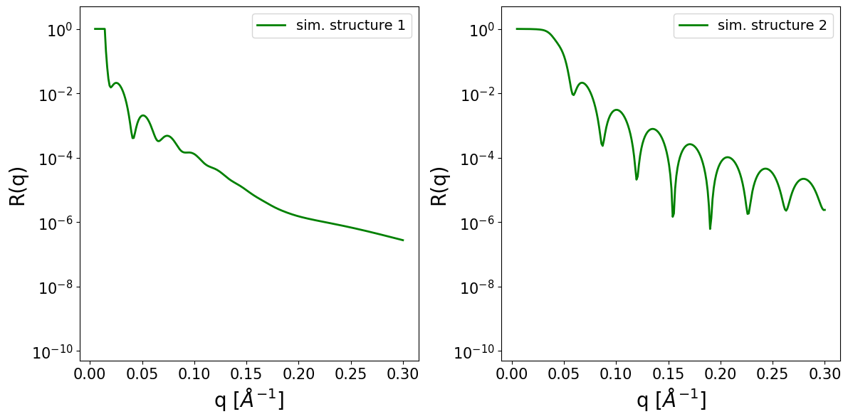
We initalize the grid of momentum transfer values (q) and the physical parameters for 2-layer structures inbetween the fronting medium (ambient) and the backing medium (substrate). Here we have a batch size of 2 (i.e. two different structures). In this example, the tensors are located on the CPU. Performing the computation on GPU ('cuda') is computationally faster for large batch sizes. Notably, we use the double-precision data types (torch.float64 for real-valued tensors or torch.complex128 for complex-valued tensors) instead of the default single-precision data type for improved accuracy.

device = torch.device('cpu') # or 'cuda'

q = torch.linspace(0.005, 0.3, 256, dtype=torch.float64, device=device)

thickness = torch.tensor([
    [30, 250], #thicknesses structure 1 (top to bottom)
    [120, 170], #thicknesses structure 2 (top to bottom)
], dtype=torch.float64, device=device)

roughness = torch.tensor([
    [3, 10, 20], #roughnesses structure 1 (top to bottom)
    [30, 5, 0], #roughnesses structure 2 (top to bottom)
], dtype=torch.float64, device=device)

sld = torch.tensor([
    [2.07, -3.47, 2.0, 6.36], #slds structure 1 (top to bottom)
    [0.0, 15, 40 + 1j*5, 20], #slds structure 2 (top to bottom)
], dtype=torch.complex128, device=device)

print(q.shape, thickness.shape, roughness.shape, sld.shape)

torch.Size([256]) torch.Size([2, 2]) torch.Size([2, 3]) torch.Size([2, 4])

The q values and the physical provided as input to the reflectivity function.

sim_reflectorch = reflectivity(
    q=q,
    thickness=thickness,
    roughness=roughness,
    sld=sld,
)

print(sim_reflectorch.shape, sim_reflectorch.dtype, sim_reflectorch.device) # shape: [batch_size, n_points]

torch.Size([2, 256]) torch.float64 cpu

Show code cell source Hide code cell source

fig, axes = plt.subplots(1,2,figsize=(12,6))
for ax in axes:
    ax.set_yscale('log')
    ax.set_ylim(0.5e-10, 5)
    ax.set_xlabel('q [$Å^{-1}$]', fontsize=20)
    ax.set_ylabel('R(q)', fontsize=20)
    ax.tick_params(axis='both', which='major', labelsize=15)
    ax.tick_params(axis='both', which='minor', labelsize=15)
    y_tick_locations = [10**(-2*i) for i in range(6)]
    ax.yaxis.set_major_locator(plt.FixedLocator(y_tick_locations))
    
axes[0].plot(q, sim_reflectorch[0], c='green', lw=2, label='sim. structure 1')
axes[1].plot(q, sim_reflectorch[1], c='green', lw=2, label='sim. structure 2')

axes[0].legend(loc='upper right', fontsize=14);
axes[1].legend(loc='upper right', fontsize=14);

plt.tight_layout()

2.2. Comparison to refnx and refl1d

We compare our reflectivity simulations with simulations performed using the well-known classical analysis packages refnx and refl1d.

2.2.1. refnx

from refnx.reflect import Slab, ReflectModel

### Structure 1
amb = Slab(thick=0, rough=0, sld=2.07)
l1 = Slab(thick=30, rough=3, sld=-3.47)
l2 = Slab(thick=250, rough=10, sld=2.0)
sub = Slab(thick=0, rough=20, sld=6.36)

structure1 = amb | l1 | l2 | sub
model1 = ReflectModel(structure1, bkg=0, dq=0)
sim_refnx_1 = model1(q.numpy())


### Structure 2
amb = Slab(thick=0, rough=0, sld=0.0)
l1 = Slab(thick=120, rough=30, sld=15)
l2 = Slab(thick=170, rough=5, sld=40+1j*5)
sub = Slab(thick=0, rough=0, sld=20)

structure2 = amb | l1 | l2 | sub
model2 = ReflectModel(structure2, bkg=0, dq=0)
sim_refnx_2 = model2(q.numpy())

Show code cell source Hide code cell source

fig, axes = plt.subplots(1,2,figsize=(12,6))
for ax in axes:
    ax.set_yscale('log')
    ax.set_ylim(0.5e-10, 5)
    ax.set_xlabel('q [$Å^{-1}$]', fontsize=20)
    ax.set_ylabel('R(q)', fontsize=20)
    ax.tick_params(axis='both', which='major', labelsize=15)
    ax.tick_params(axis='both', which='minor', labelsize=15)
    y_tick_locations = [10**(-2*i) for i in range(6)]
    ax.yaxis.set_major_locator(plt.FixedLocator(y_tick_locations))
    
axes[0].plot(q, sim_reflectorch[0], c='yellow', lw=4, label='sim. reflectorch structure 1')
axes[0].plot(q.numpy(), sim_refnx_1, c='red', lw=1, ls='--', label='sim. refnx structure 1')

axes[1].plot(q, sim_reflectorch[1], c='yellow', lw=4, label='sim. reflectorch structure 2')
axes[1].plot(q.numpy(), sim_refnx_2, c='red', lw=1, ls='--', label='sim. refnx structure 2')

axes[0].legend(loc='upper right', fontsize=14);
axes[1].legend(loc='upper right', fontsize=14);

plt.tight_layout()

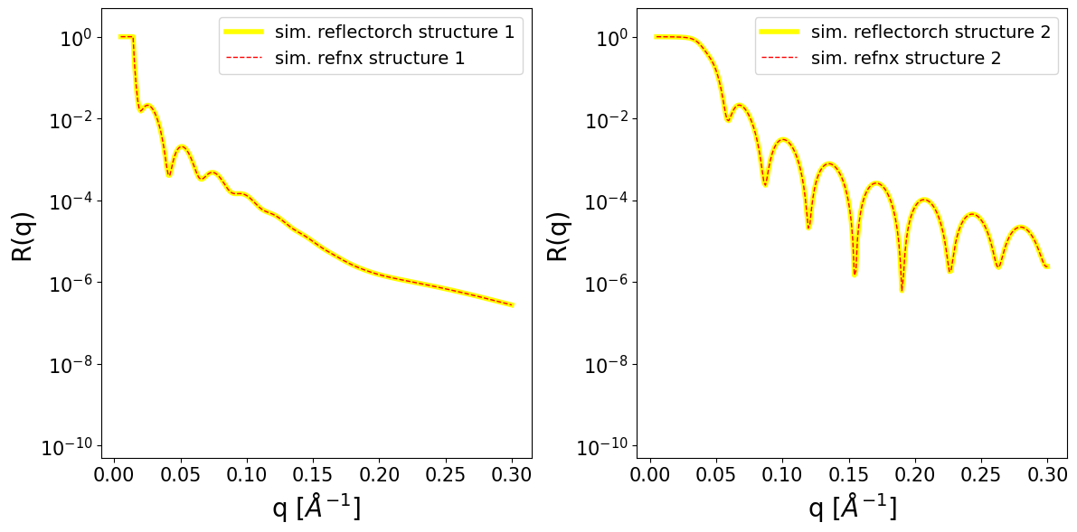
print(f'Maximum relative difference (sim 1): {(np.abs((sim_reflectorch[0].numpy() - sim_refnx_1)) / sim_refnx_1).max()}')
print(f'Maximum relative difference (sim 2): {(np.abs((sim_reflectorch[1].numpy() - sim_refnx_2)) / sim_refnx_2).max()}')

Maximum relative difference (sim 1): 2.5179880710123875e-15
Maximum relative difference (sim 2): 5.044054966894104e-15

2.2.2. refl1d

import refl1d
import refl1d.names

probe = refl1d.names.QProbe(
    Q=q.numpy(),
    dQ=np.zeros_like(q),
)

### Structure 1
sld_amb = refl1d.names.SLD(rho=2.07)
sld_l1 = refl1d.names.SLD(rho=-3.47)
sld_l2 = refl1d.names.SLD(rho=2.0)
sld_sub = refl1d.names.SLD(rho=6.36)

structure1 = sld_sub(0, 20) | sld_l2(250, 10) | sld_l1(30, 3) | sld_amb(0, 0) ### in refl1d the layer order is from substrate to ambient
experiment1 = refl1d.names.Experiment(probe=probe, sample=structure1)
sim_refl1d_1 = experiment1.reflectivity()[1]

### Structure 2
sld_amb = refl1d.names.SLD(rho=0)
sld_l1 = refl1d.names.SLD(rho=15)
sld_l2 = refl1d.names.SLD(rho=40, irho=5)
sld_sub = refl1d.names.SLD(rho=20)

structure2 = sld_sub(0, 0) | sld_l2(170, 5) | sld_l1(120, 30) | sld_amb(0, 0)
experiment2 = refl1d.names.Experiment(probe=probe, sample=structure2)
sim_refl1d_2 = experiment2.reflectivity()[1]

Show code cell source Hide code cell source

fig, axes = plt.subplots(1,2,figsize=(12,6))
for ax in axes:
    ax.set_yscale('log')
    ax.set_ylim(0.5e-10, 5)
    ax.set_xlabel('q [$Å^{-1}$]', fontsize=20)
    ax.set_ylabel('R(q)', fontsize=20)
    ax.tick_params(axis='both', which='major', labelsize=15)
    ax.tick_params(axis='both', which='minor', labelsize=15)
    y_tick_locations = [10**(-2*i) for i in range(6)]
    ax.yaxis.set_major_locator(plt.FixedLocator(y_tick_locations))
    
axes[0].plot(q, sim_reflectorch[0], c='yellow', lw=4, label='sim. reflectorch structure 1')
axes[0].plot(q.numpy(), sim_refl1d_1, c='blue', lw=1, ls='-.', label='sim. refl1d structure 1')

axes[1].plot(q, sim_reflectorch[1], c='yellow', lw=4, label='sim. reflectorch structure 2')
axes[1].plot(q.numpy(), sim_refl1d_2, c='blue', lw=1, ls='-.', label='sim. refl1d structure 2')

axes[0].legend(loc='upper right', fontsize=14);
axes[1].legend(loc='upper right', fontsize=14);

plt.tight_layout()

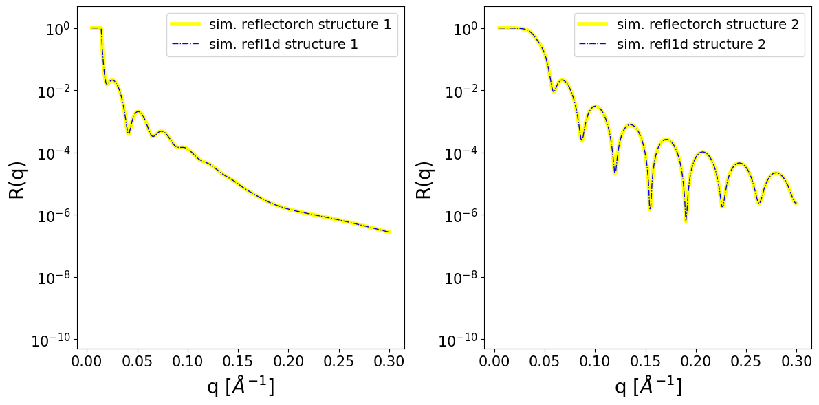
print(f'Maximum relative difference (sim 1): {(np.abs((sim_reflectorch[0].numpy() - sim_refl1d_1)) / sim_refl1d_1).max()}')
print(f'Maximum relative difference (sim 2): {(np.abs((sim_reflectorch[1].numpy() - sim_refl1d_2)) / sim_refl1d_2).max()}')

Maximum relative difference (sim 1): 1.0018470239619891e-13
Maximum relative difference (sim 2): 4.6703425310918357e-14

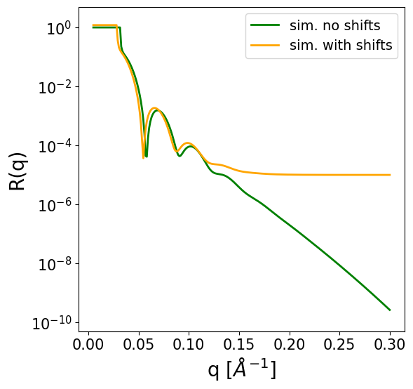
2.3. Incorporating experimental artifacts

We can incorporate the effects of experimental misalignment (q offset, intensity normalization error) as well as a constant background (relevant in neutron experiments), by providing the following optional arguments to the reflectivity function (either as a float or as a tensor of shape [batch_size, 1]):

• q_shift: the offset in q due to misalignment

• r_scale: a multiplication factor for scaling the intensity of the reflectivity curve

• background: the constant background added to the reflectivity curve

device = torch.device('cpu')

q = torch.linspace(0.005, 0.3, 256, dtype=torch.float64, device=device)

thickness = torch.tensor([[60, 120]], dtype=torch.float64, device=device)
roughness = torch.tensor([[20, 40, 10]], dtype=torch.float64, device=device)
sld = torch.tensor([[15, 10, 20]], dtype=torch.float64, device=device)

sim = reflectivity(q=q, thickness=thickness, roughness=roughness, sld=sld)
sim_shifts = reflectivity(q=q, thickness=thickness, roughness=roughness, sld=sld, 
                          q_shift=0.003, r_scale=1.2, background=10**(-5))

Show code cell source Hide code cell source

fig, ax = plt.subplots(1,1,figsize=(6,6))

ax.set_yscale('log')
ax.set_ylim(0.5e-10, 5)
ax.set_xlabel('q [$Å^{-1}$]', fontsize=20)
ax.set_ylabel('R(q)', fontsize=20)
ax.tick_params(axis='both', which='major', labelsize=15)
ax.tick_params(axis='both', which='minor', labelsize=15)
y_tick_locations = [10**(-2*i) for i in range(6)]
ax.yaxis.set_major_locator(plt.FixedLocator(y_tick_locations))

ax.plot(q, sim[0], c='green', lw=2, label='sim. no shifts')
ax.plot(q, sim_shifts[0], c='orange', lw=2, label='sim. with shifts')

ax.legend(loc='upper right', fontsize=14);

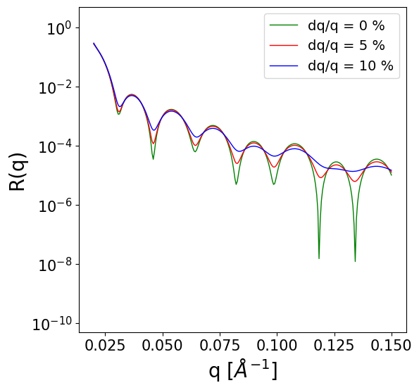
2.4. Resolution smearing

In real experiments (particularly for neutrons) the measured reflectivity curves are smeared due to finite resolution in the incident angle and beam energy (which gives a finite resolution in the momentum transfer q).

In order to apply resolution smearing, the reflectivity function takes the following optional arguments:

• dq - a tensor containing the smearing coefficients. It has shape [batch_size, 1] for linear and constant smearing, or [batch_size, num_points] for pointwise smearing.

• constant_dq - a boolean flag to switch between linear and constant smearing

• gauss_num - the number of points used to define the Gaussian smearing kernel. A higher number increases precision at the cost of computational efficiency

2.4.1. Linear (and constant) smearing

If dq is a tensor of shape [batch_size, 1] and constant_dq is False (default case), linear smearing if performed (typical for neutron experiments). In this case, the meaning of the values in the tensor dq are not actually dq, but the resolutions s=dq/q for each curve (such that dq=s*q).

Alternatively, if dq is a tensor of shape [batch_size, 1] and constant_dq is True, constant smearing is performed (sometimes used for x-ray experiments). In this case, the meaning of the values in the tensor are the constant dq for each curve.

device = torch.device('cpu')
q = torch.linspace(0.02, 0.15, 256, dtype=torch.float64, device=device)

thickness = torch.tensor([
    [200, 150],
    [200, 150],
], dtype=torch.float64, device=device)

roughness = torch.tensor([
    [1, 5, 2],
    [1, 5, 2],
], dtype=torch.float64, device=device)

sld = torch.tensor([
    [4, 2, 6.5],
    [4, 2, 6.5],
], dtype=torch.float64, device=device)

#Two different resolution coefficients for linear smearing (dq/q = 0.05 (5%) and dq/q = 0.1 (10%))

dq = torch.tensor([
    [0.05],
    [0.1],
], dtype=torch.float64, device=device)

print(f'Shape dq: {dq.shape}')

sim_smearing = reflectivity(
    q=q, 
    thickness=thickness, 
    roughness=roughness, 
    sld=sld,
    dq=dq,
    gauss_num=51,
    constant_dq=False,
)

#We compute the unsmeared curve (dq/q=0) separately
sim_no_smearing = reflectivity(
    q=q, 
    thickness=thickness, 
    roughness=roughness, 
    sld=sld,
)

Shape dq: torch.Size([2, 1])

Show code cell source Hide code cell source

fig, ax = plt.subplots(1,1,figsize=(6,6))
ax.set_yscale('log')
ax.set_ylim(0.5e-10, 5)
ax.set_xlabel('q [$Å^{-1}$]', fontsize=20)
ax.set_ylabel('R(q)', fontsize=20)
ax.tick_params(axis='both', which='major', labelsize=15)
ax.tick_params(axis='both', which='minor', labelsize=15)
y_tick_locations = [10**(-2*i) for i in range(6)]
ax.yaxis.set_major_locator(plt.FixedLocator(y_tick_locations))
    
ax.plot(q, sim_no_smearing[0], c='g', lw=1, label='dq/q = 0 %')
ax.plot(q, sim_smearing[0], c='r', lw=1, label=f'dq/q = {int(100*dq[0].item())} %')
ax.plot(q, sim_smearing[1], c='b', lw=1, label=f'dq/q = {int(100*dq[1].item())} %')

ax.legend(loc='upper right', fontsize=14);

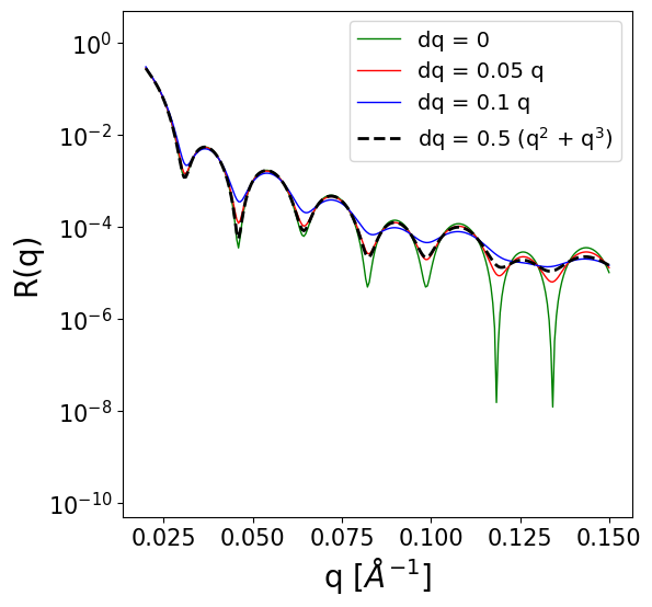
2.4.2. Pointwise smearing

If dq is a tensor of shape [batch_size, num_points], pointwise smearing is performed. This is more general, as dq can be an arbitrary function of q, but it is also more computationally expensive.

thickness = torch.tensor([
    [200, 150],
], dtype=torch.float64, device=device).repeat(4, 1)

roughness = torch.tensor([
    [1, 5, 2],
], dtype=torch.float64, device=device).repeat(4, 1)

sld = torch.tensor([
    [4, 2, 6.5],
], dtype=torch.float64, device=device).repeat(4, 1)

dq_no_smearing = torch.zeros_like(q)
dq_linear_5 = 0.05 * q
dq_linear_10 = 0.1 * q
dq_arbitrary = 0.5*(q**2 + q**3)

dq = torch.stack([
    dq_no_smearing,
    dq_linear_5,
    dq_linear_10,
    dq_arbitrary,
], dim=0)

print(f'Shape dq: {dq.shape}')

sim_smearing_pointwise = reflectivity(
    q=q, 
    thickness=thickness, 
    roughness=roughness, 
    sld=sld,
    dq=dq,
    gauss_num=51,
)

Shape dq: torch.Size([4, 256])

Show code cell source Hide code cell source

fig, ax = plt.subplots(1,1,figsize=(6,6))
ax.set_yscale('log')
ax.set_ylim(0.5e-10, 5)
ax.set_xlabel('q [$Å^{-1}$]', fontsize=20)
ax.set_ylabel('R(q)', fontsize=20)
ax.tick_params(axis='both', which='major', labelsize=15)
ax.tick_params(axis='both', which='minor', labelsize=15)
y_tick_locations = [10**(-2*i) for i in range(6)]
ax.yaxis.set_major_locator(plt.FixedLocator(y_tick_locations))
    
ax.plot(q, sim_smearing_pointwise[0], c='g', lw=1, label='dq = 0')
ax.plot(q, sim_smearing_pointwise[1], c='r', lw=1, label=f'dq = 0.05 q')
ax.plot(q, sim_smearing_pointwise[2], c='b', lw=1, label=f'dq = 0.1 q')
ax.plot(q, sim_smearing_pointwise[3], c='black', lw=2, ls='--', label=f'dq = 0.5 (q$^2$ + q$^3$)')

ax.legend(loc='upper right', fontsize=14);